


 (C:)
(C:) cs300
cs300
Database
Alongside compilers and operating systems, the DB is arguably one of the most fascinating pieces of systems software (§603) ever built. It packs an extraordinary density of CS subfields into a single system, from relational algebra and B-tree indexing to write-ahead logging, multiversion concurrency control, query optimisation (which is essentially a compiler problem), and distributed consensus. Nearly every non-trivial application depends on one.
I
1.1. Relational Model
A database (DB) is a structured collection of persistent data managed by a system that supports efficient retrieval and modification. Databases have historically exceeded main memory capacity. RAM (§601#1.3) in the 1960s–70s was measured in kilobytes, so the authoritative copy of data lived on disk, with memory serving only as a buffer. Early navigational databases such as IBM’s IMS (1966) and the CODASYL network model (1969) stored data in hierarchical or graph structures that programs traversed via linked pointers. Because programs referenced data by its physical address on disk, any storage reorganisation broke existing code.
Edgar Codd’s relational model (1970) broke this coupling by proposing that data be organised as relations, sets of tuples over named attributes, manipulated through a closed algebra of operations (e.g. select, project, join) rather than procedural navigation. The model established data independence, separating logical structure from physical storage so that the engine could reorganise data without breaking applications. IBM’s System R and UC Berkeley’s Ingres (both 1974) were the first relational database management systems (RDBMS) to demonstrate the model’s practicality.
In particular, System R introduced structured query language (SQL), a DSL for querying and managing relational databases (§602#2.2), where one specifies “what” data to retrieve or modify and the engine determines “how” to execute it efficiently. This separation of specification from execution enables query optimisation, since the engine can choose among equivalent strategies without changing semantics. Ingres, led by Michael Stonebraker (Turing Award, 2014), spawned a successor project called Postgres (1986), whose Postgres95 release replaced its POSTQUEL query language with SQL (1995) before the rename to PostgreSQL (1996), which remains the reference open-source RDBMS.
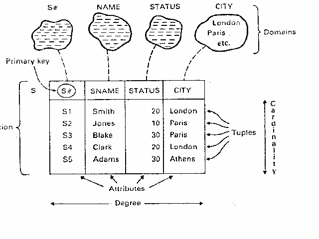
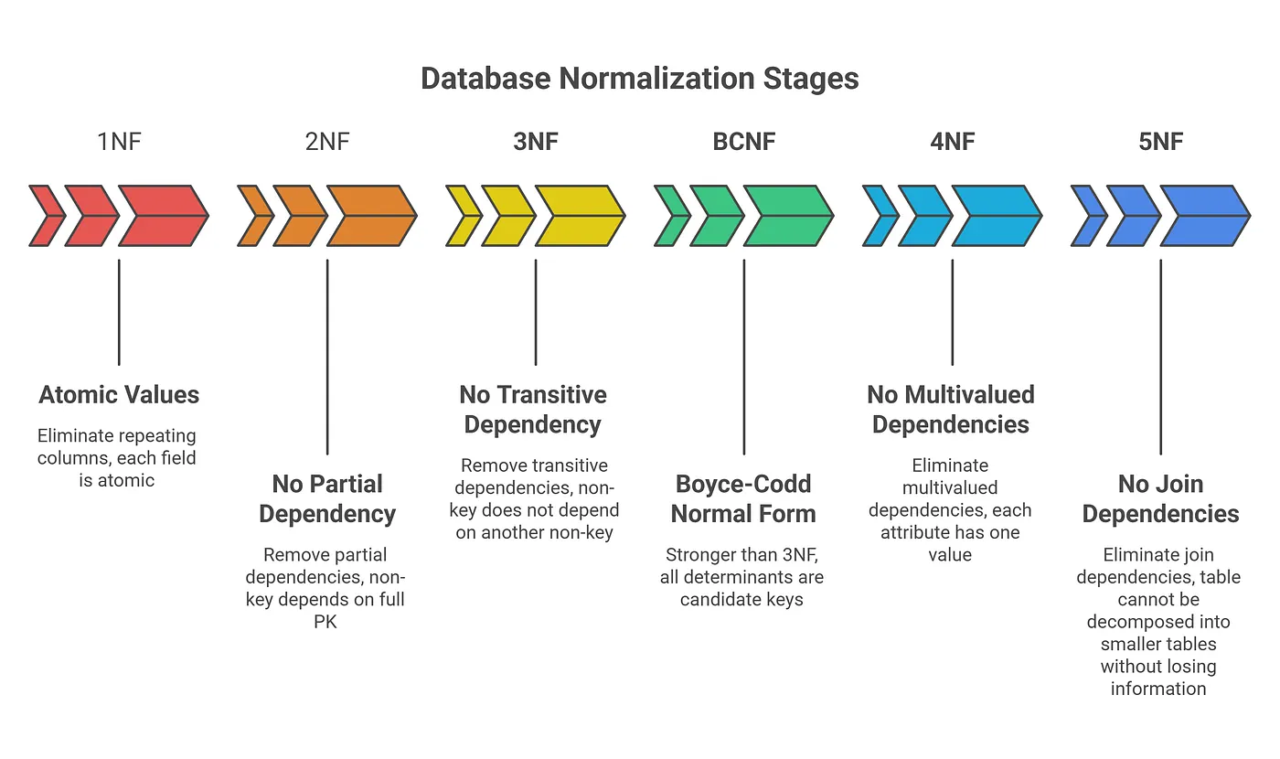
Practitioners refer to relations as tables, tuples as rows, and attributes as columns. Each table is defined by a schema that specifies column names, data types, and constraints. Primary keys (pk) uniquely identify rows and may span multiple columns (composite key), and foreign keys (fk) enforce referential integrity by requiring that a value in one table correspond to an existing primary key in another. Normalisation decomposes tables to eliminate redundancy and update anomalies. A functional dependency $X \to Y$ holds when any two rows agreeing on attributes $X$ agree on $Y$, and successive normal forms (1NF through BCNF) impose progressively stricter constraints on where such dependencies may sit, BCNF requiring every determinant $X$ to be a superkey. Denormalisation deliberately reintroduces redundancy to optimise read performance for specific query patterns, at the cost of increased storage and write complexity.
1.2. Storage Engine
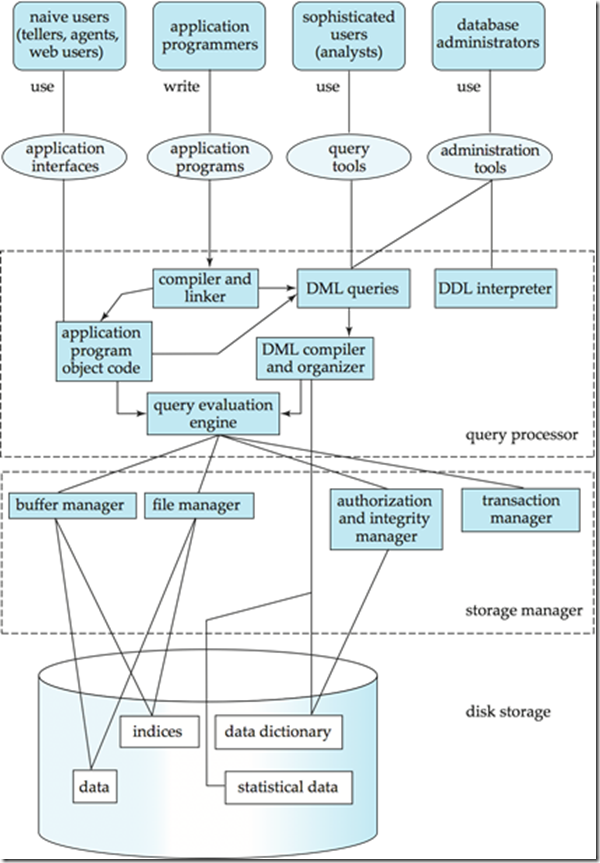
The relational model is a logical abstraction. The storage manager (aka. storage engine), the DBMS component responsible for data transfer between disk and memory, materialises relations on disk and serves them back efficiently. Since disk I/O (§601#1.4) is orders of magnitude slower than memory access, the storage manager’s design is oriented around minimising it. Data is organised into fixed-size pages (8 KB in PostgreSQL, 16 KB in InnoDB) aligned with the disk’s block-oriented access, so every I/O transfers a useful unit of work. A buffer pool caches recently accessed pages in memory, an approach Gray’s five-minute rule (1987) formalised economically: if a page is accessed more often than once every five minutes, keeping it resident is cheaper than re-reading it. The buffer pool deliberately duplicates the role of the OS page cache (§603#3.2), since the engine must control eviction itself (PostgreSQL approximates LRU with a clock-sweep) and must guarantee that a dirty page reaches disk only after its WAL records do (§2.3), an ordering the kernel’s opaque write-back cannot promise.
In PostgreSQL, a database cluster is the top-level directory (PGDATA), each database is a subdirectory under base/ identified by OID, and each table is stored as one or more heap files named by the table’s OID. A heap file is a sequence of 8 KB pages, each containing multiple tuples. Each tuple is preceded by a 23-byte header (padded to 24 by alignment) containing transaction visibility fields (xmin, xmax), a tuple identifier (ctid, pointing to the row’s physical location as a page/offset pair), and an infomask encoding null flags, lock state, and hint bits. This header makes MVCC possible at the storage level, since the engine can determine visibility without consulting a separate structure. Values exceeding approximately 2 KB are compressed and moved out-of-line by the oversized-attribute storage technique (TOAST) into a companion table, keeping the main heap pages compact.
Data layout can follow two fundamentally different orientations driven by workload. Online Transaction Processing (OLTP) workloads read and write individual records, while Online Analytical Processing (OLAP) workloads aggregate millions of rows over a few columns. The former favours the N-ary Storage Model (NSM, row-oriented) where all columns of a row sit contiguously so that a single page read retrieves the full record. The latter favours the Decomposition Storage Model (DSM, column-oriented) where values of the same column are stored together, enabling aggressive compression and vectorised scans. PostgreSQL uses NSM; Redshift uses DSM, yet both share the same SQL interface and PostgreSQL wire protocol, since Redshift forked from PostgreSQL 8.0 but replaced the storage engine entirely with a columnar, MPP architecture from ParAccel.
1.3. Indexing
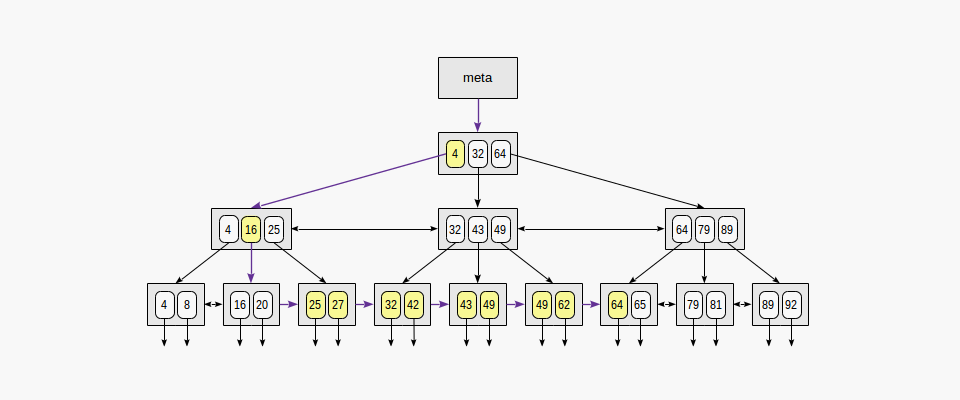
Without an index, every lookup requires a sequential scan of the entire heap. An index maps search keys to the physical locations of matching rows, trading write overhead for read speed. The simplest indexing structure is a binary search tree (BST): it narrows the search space by half at each level, giving $O(\log_2 n)$ node visits. But each visit is a separate disk read, so a billion-key BST requires roughly 30 I/Os per lookup, far too many when each I/O costs milliseconds. The B-tree (Bayer and McCreight, 1972) solves this by exploiting the disk’s block-oriented access: each node holds up to $m - 1$ keys and $m$ child pointers and maps to one page, so a single I/O retrieves an entire node and the height drops to 3-4 levels.
The B+ tree refines the B-tree by restricting row pointers to leaf nodes (internal nodes hold only keys for routing) and linking leaves via sibling pointers for sequential range scans. Insertion costs $O(\log_b n)$ worst case for the search, while the splits that propagate upward to maintain balance are $O(1)$ amortised. With a branching factor $b$ (typically in the hundreds, since one node fits one page) and $n$ keys, a B+ tree has height $O(\log_b n)$, so even tables with billions of rows require only 3-4 page reads per lookup.
Hash indexes provide $O(1)$ average-case point lookups but cannot serve range queries or ordered iteration. Composite indexes on multiple columns $(c_1, c_2, \ldots, c_k)$ satisfy queries that filter on a leftmost prefix of the indexed columns. A covering index includes all columns a query needs, allowing the engine to answer entirely from the index without touching the heap (an index-only scan). PostgreSQL also offers specialised access methods beyond B+ tree: GIN (Generalised Inverted Index) for full-text search and JSONB containment, GiST (Generalised Search Tree) for geometric and range types, SP-GiST (Space-Partitioned GiST) for space-partitioned structures, and BRIN (Block Range Index) for large, naturally ordered tables where storing min/max values per consecutive block range yields an index orders of magnitude smaller than a full B+ tree.
Indexes are not free. Every INSERT, UPDATE, or DELETE must maintain every index on the table, not just the heap. In PostgreSQL, indexes store pointers to all tuple versions including dead ones, so index bloat accumulates between VACUUM cycles and may eventually require REINDEX. The query planner chooses between an index scan and a sequential scan based on estimated selectivity $s \in [0, 1]$: when $s$ is low (few matching rows), the index avoids reading irrelevant pages; when $s$ is high, a sequential scan is cheaper because it reads pages contiguously rather than issuing random I/O. The planner models this tradeoff via random_page_cost and seq_page_cost (default ratio 4:1 for spinning disks, often set to 1.1:1 for SSDs).
- …
II
2.1. ACID
The storage layer so far assumes a single user. When multiple transactions access the same data concurrently, the system needs formal guarantees about correctness. A transaction groups one or more operations into a logical unit of work satisfying the ACID properties, articulated by Jim Gray (Turing Award, 1998) and named by Härder and Reuter (1983): atomicity (all-or-nothing execution), consistency (valid state to valid state), isolation (concurrent transactions do not observe intermediate states), and durability (committed effects survive crashes). Each property has a cost. Atomicity requires an undo mechanism, durability requires forcing writes to stable storage, and strict isolation reduces concurrency.
Of the four properties, consistency stands apart. Atomicity, isolation, and durability are guarantees the database engine enforces mechanically, but consistency depends on the application defining correct invariants through constraints (NOT NULL, UNIQUE, CHECK, foreign keys) and transaction logic. A transfer that debits one account without crediting another violates consistency even if the transaction commits atomically. In practice, isolation is the most negotiable property, since full serialisability is expensive and most workloads tolerate weaker guarantees in exchange for higher throughput.
2.2. Concurrency Control
The simplest way to guarantee isolation is to execute transactions serially, but serial execution forfeits concurrency. The challenge is to run transactions concurrently while producing results equivalent to some serial order, a property with a checkable criterion, since a schedule is conflict-serialisable if and only if its precedence graph (i.e. nodes are transactions, with an edge $T_i \to T_j$ whenever an operation of $T_i$ conflicts with and precedes one of $T_j$) is acyclic, the correctness counterpart of the deadlock cycle in §604#3.4. Isolation levels formalise how much concurrency a system permits by relaxing this guarantee. Read Uncommitted allows dirty reads (seeing uncommitted writes). Read Committed (PostgreSQL’s default) prevents dirty reads but permits non-repeatable reads (a row changes between two reads within the same transaction). Repeatable Read prevents both but may allow phantom reads under the ANSI standard (new rows appearing in a range query); PostgreSQL’s Repeatable Read already prevents phantoms via snapshot isolation, so its Serialisable level (SSI, below) targets write skew and other serialisation anomalies instead.
Two-phase locking (2PL), introduced in System R, is the classical enforcement mechanism: a transaction acquires locks before accessing data (growing phase) and releases them only after committing or aborting (shrinking phase). This guarantees serialisability but causes deadlocks and reduces concurrency, since readers block writers and vice versa. Multiversion concurrency control (MVCC), pioneered by Reed (1978) and adopted by PostgreSQL, MySQL/InnoDB, and Oracle, adopts a different strategy. Each write creates a new version of the row rather than overwriting in place, and each transaction sees a consistent snapshot of the database as of its start time. Readers never block writers and writers never block readers, which is why MVCC dominates in practice.
In PostgreSQL, MVCC is implemented at the storage level through the heap tuple header. Each row version is stamped with xmin (the creating transaction ID) and xmax (the deleting or locking transaction ID). A transaction’s snapshot records the set of in-progress transaction IDs at snapshot time, and a row version is visible if its xmin has committed and its xmax has not. An UPDATE does not modify the existing tuple; it inserts a new version and sets xmax on the old one, leaving dead tuples that VACUUM must eventually reclaim. Autovacuum runs VACUUM automatically based on configurable thresholds. Because transaction IDs are 32-bit integers with a $2^{31}$ visibility horizon, PostgreSQL also requires periodic anti-wraparound vacuuming to freeze old transaction IDs, and failure to vacuum can force the database into read-only mode. MySQL/InnoDB implements MVCC differently, using undo logs to reconstruct older versions on demand from a single physical copy, avoiding dead-tuple accumulation but requiring undo log purging.
At the strongest isolation level, PostgreSQL implements Serialisable Snapshot Isolation (SSI, Cahill et al. 2008), which detects dangerous patterns of read-write dependencies between concurrent transactions and aborts one to prevent anomalies, rather than acquiring predicate locks that would block concurrent access. SSI makes PostgreSQL’s SERIALIZABLE level practical, since it preserves the non-blocking property of snapshot isolation while guaranteeing full serialisability.
2.3. Write-Ahead Logging
Write-ahead logging (WAL) is the mechanism that provides atomicity and durability. Before any modification is applied to a data page, a log record describing the change is first written to a sequential, append-only log on stable storage. If the system crashes, committed changes can be replayed from the log; uncommitted changes are rolled back. Because the log is written sequentially, it is far cheaper than random writes to scattered data pages (§601#1.4), and the database can batch multiple transactions’ log records into a single fsync() via group commit.
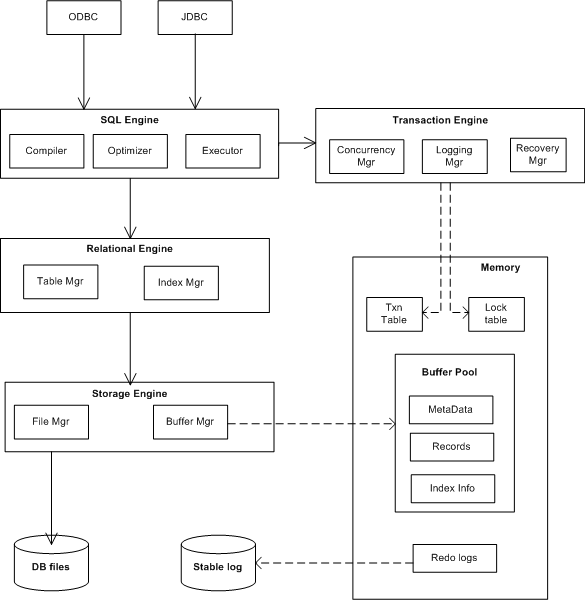
In PostgreSQL, WAL records are written to 16 MB segment files in pg_wal/ (formerly pg_xlog/). During normal operation, modified (“dirty”) pages accumulate in the buffer pool and are flushed to disk lazily by the background writer and checkpointer, but only after their corresponding WAL records have reached stable storage (the WAL-before-data rule). A checkpoint periodically forces all dirty pages to disk and records the log sequence number (LSN) at which recovery can begin, bounding the amount of WAL that must be replayed after a crash. The WAL also enables streaming replication: a standby server continuously receives and replays WAL segments from the primary, maintaining a near-real-time copy. Logical replication (PostgreSQL 10+) decodes the WAL into logical change events, enabling selective replication of individual tables or cross-version upgrades.
On crash recovery, the database replays the WAL from the last checkpoint forward. The redo phase reapplies all changes (committed or not) that may not have reached the data files, restoring the database to the exact state at the moment of the crash. PostgreSQL then identifies transactions that were in progress at crash time and marks them as aborted, so their effects become invisible through normal MVCC visibility rules rather than requiring an explicit undo phase. This is possible because PostgreSQL’s MVCC never overwrites data in place, so “undoing” an uncommitted transaction simply means its row versions are never visible to any future snapshot. File system journaling (e.g. ext3, 2001) adopted the same principle for metadata consistency.
III
3.1. Structured Query Language
Codd’s original algebra operates on sets with no concept of missing values or ordering. SQL is relationally complete w.r.t. this algebra, but departs from it in three practical ways: i) it operates on bags (i.e. multisets with duplicates) rather than sets to minimise the cost of deduplicating all intermediaries; ii) it introduces NULL to represent missing or unknown values, which requires three-valued logic (i.e. TRUE, FALSE, UNKNOWN) as any comparison involving NULL yields UNKNOWN; and iii) it adds ORDER BY to impose a sequence on inherently unordered relations; DISTINCT serves as the explicit operator to recover set semantics when needed.
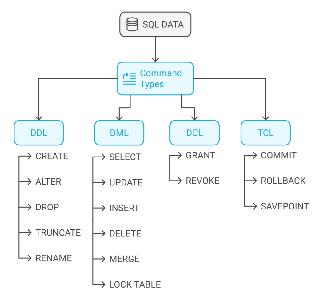
SQL is standardised by ISO/IEC and revised periodically: adding recursive queries (SQL:1999), window functions (SQL:2003), JSON support (SQL:2016), and property graph queries (SQL:2023). SQL statements are often classified into: i) Data manipulation language (DML) for reading / writing data; ii) Data definition language (DDL) for defining / modifying schema; iii) Data control language (DCL) for managing permissions; and iv) Transaction control language (TCL) for demarcating transaction boundaries. Only DML passes through the optimiser (§3.2). In practice, however, each RDBMS carries a dialect with vendor-specific extensions and omissions.
These successive revisions have also extended SQL beyond the original algebra, which include adding aggregation (e.g. GROUP BY with aggregate functions, filtered by HAVING), subqueries (e.g. scalar, correlated, and EXISTS predicates), common table expressions (e.g. WITH clauses, including recursive CTEs for hierarchical queries), and window functions (e.g. OVER/PARTITION BY for running totals, ranks, and moving averages without collapsing rows). These constructs compose along SQL’s logical evaluation order: FROM $\to$ WHERE $\to$ GROUP BY $\to$ HAVING $\to$ SELECT $\to$ ORDER BY, where each stage consumes the previous relation.
3.2. Query Processor
The compilation pipeline that turns a SQL statement into executable operations mirrors a compiler (§602#2.2): a parser (generated from a Bison grammar in PostgreSQL, gram.y) validates syntax and produces an AST, a binder (called the analyser in PostgreSQL) resolves names against the catalogue (the database’s metadata store of schemas, tables, columns, and constraints), and a logical planner translates the AST into a tree of relational algebra operators. PostgreSQL inserts an additional rewriter stage (pg_rewrite_query) between analysis and planning that expands views (i.e. named queries stored in the catalogue and referenced like tables), applies rule-based transformations, and enforces row-level security policies. This pipeline is not unique to databases; engines such as SparkSQL (Catalyst) reuse the same architecture to optimise relational algebra over DataFrames rather than stored tables.
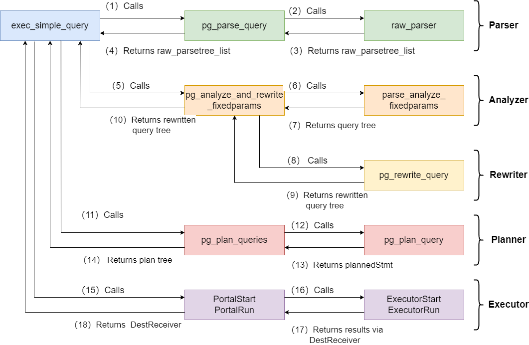
The logical planner produces a tree of relational algebra operators, selection $\sigma$, projection $\pi$, and join $\bowtie$, so a SELECT-FROM-WHERE compiles to $\pi(\sigma(R \bowtie S))$, but the same query admits many equivalent trees with orders-of-magnitude difference in cost. System R (1979) introduced the first cost-based optimiser, treating plan selection as a search problem over equivalent expressions, an insight that made SQL practical and that every modern engine still follows. The optimiser applies equivalence-preserving transformations such as predicate pushdown ($\sigma_\theta(R \bowtie S) = R \bowtie \sigma_\theta(S)$ when $\theta$ references only $S$’s attributes), join reordering, and projection pruning, then the physical planner maps each logical operator to a concrete algorithm and estimates cost using statistics maintained on tables and columns.
PostgreSQL stores these in pg_statistic (histograms, most-common-value lists, distinct counts), updated by the ANALYZE command (run automatically by autovacuum). Cardinality estimation, predicting how many rows an operator will produce, is inherently imprecise, and errors compound multiplicatively across joins. The primary source of error is the independence assumption (that column values are uncorrelated); PostgreSQL 10+ added multivariate statistics (CREATE STATISTICS) to model correlations between columns. The quality of the cardinality estimator remains the single largest determinant of plan quality in practice.
EXPLAIN ANALYZE exposes the planner’s chosen plan alongside actual execution statistics (rows, time, buffers), though its cost metric is an abstract unit rather than wall-clock time, and the BUFFERS option is needed to distinguish cache hits from disk reads. In production, auto_explain captures plans of actual slow queries without manual intervention, and pg_stat_statements tracks cumulative execution statistics (calls, total time, rows) per normalised query, making it the starting point for identifying slow queries.
Join algorithms illustrate the range of physical operators. A nested loop join iterates over the outer relation and probes the inner for each row ($O(n \cdot m)$), benefiting from an index on the inner side. A hash join builds a hash table on the smaller relation and probes it with the larger ($O(n + m)$ expected), preferred when no useful index exists. A sort-merge join sorts both relations on the join key and merges them in a single pass, performing well when inputs are already sorted or when the result must be ordered. PostgreSQL’s planner evaluates all applicable algorithms for each join and selects the cheapest based on its cost model. Join ordering is NP-hard, and System R’s dynamic programming approach is exponential ($O(2^n)$ subsets) in the number of joined tables; when this becomes intractable, PostgreSQL falls back to a GEnetic query optimiser (GEQO) (e.g. geqo_threshold = 12, default).
- …
Once the planner selects a plan, the executor runs it. The classical execution model is the volcano (iterator) model (Graefe, 1994), where each operator implements an open(), next(), close() interface. Operators compose into a tree, and calling next() on the root pulls one tuple at a time through the pipeline. PostgreSQL uses this model, which supports pipelining (producing output before consuming all input), but incurs per-tuple function-call and interpretation overhead that becomes significant on analytical workloads scanning millions of rows.
Vectorised execution (e.g. DuckDB, ClickHouse) amortises this overhead by processing batches of tuples (typically 1024-4096) per next() call, enabling SIMD instructions and better cache utilisation. PostgreSQL’s built-in operators and extension functions (e.g. pgvector’s distance computations) are ahead-of-time compiled C, but the expression evaluator that combines them is interpreted. Parallel query execution partitions work across multiple workers, with the exchange (Gather) operator redistributing intermediate tuples between parallel pipeline segments. PostgreSQL supports intra-query parallelism for sequential scans, hash joins, and aggregations since version 9.6.
- …
3.3. Process-per-Connection
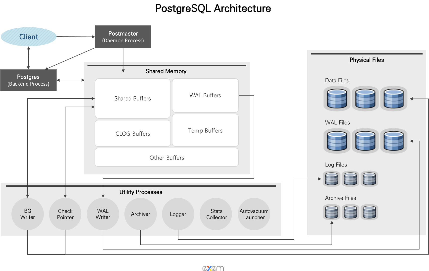
Everything covered so far, the storage engine (§I), transaction manager (§II), and query processor (§3.1–3.2), executes inside a single PostgreSQL backend process. The backend reads and writes data pages through a shared buffer pool, appends change records to shared WAL buffers, and coordinates with other backends via shared lock tables, all mapped into a single shared memory segment. Outside the backend, utility processes handle maintenance asynchronously: the background writer and checkpointer flush dirty pages (§2.3), the WAL writer flushes WAL buffers, the archiver ships completed WAL segments, and the autovacuum launcher reclaims dead tuples (§2.2).
The segment is sized once at startup, chiefly by shared_buffers, and cannot grow. Parallel query is the exception, as worker backends exchange tuples through additional POSIX shared memory created at runtime under /dev/shm. Containers starve exactly this kind, since Docker and Kubernetes default that tmpfs to 64 MB (§607#2.1), so a parallel hash join that spills past it fails with “could not resize shared memory segment”, a limit raised with –shm-size or an in-memory emptyDir, or avoided by lowering work_mem and parallelism.
PostgreSQL uses a process-per-connection model (§604#2.1), an architectural choice inherited from 1980s Unix where threads were not portable and process isolation ensured that a crash in one backend could not corrupt another. The postmaster calls fork() to create a dedicated backend process for each new connection. MySQL (1995), born after threads became portable, instead serves each connection with a thread inside one process (§604#2.2), trading crash isolation for cheaper connections and shared caches. In PostgreSQL, then, the number of concurrent connections directly determines how many OS processes compete for hardware. A consequence of this isolation is that each backend compiles and caches query plans independently; Oracle and SQL Server, by contrast, maintain a shared plan cache across sessions, amortising compilation cost for repeated queries.
Each fork() duplicates the parent’s page table via copy-on-write and allocates a new task_struct, stack, and kernel resources (§603#3.1). A backend’s private memory, including work_mem for sorts and hash tables, maintenance_work_mem for VACUUM and index builds, and the plan cache, is not shared and scales linearly with connection count. Context switches between backends are inter-process (§603#3.1), requiring a page-table swap (CR3 write) and TLB flush, rather than the cheaper intra-thread register swap. With hundreds of backends, the scheduler spends measurable time on these switches and the resulting cache pollution (§603#3.1), which is precisely the overhead the USL’s $\beta$ term captures.
Once active connections exceed what the hardware can service, processes contend for cores and disk bandwidth. The Universal Scalability Law (USL, 1993) formalises this: $C(N) = N / (1 + \alpha(N-1) + \beta N(N-1))$, where $\alpha$ captures serialisation (Amdahl) and $\beta$ captures coherence (cross-process coordination such as lock contention and cache invalidation). The $\beta$ term causes throughput to decline past an optimal $N$, not merely plateau. The PostgreSQL community’s pool sizing heuristic $\text{pool size} = 2C + D$, where $C$ is CPU cores and $D$ is effective disk spindles (approaching 0 for SSDs), deliberately keeps pools small. HikariCP popularised this formula, demonstrating empirically that a 4-core SSD server with ~9 connections outperforms one with hundreds. The demand side follows from Little’s Law, $L = \lambda W$ ($L$ = concurrent connections, $\lambda$ = TPS, $W$ = average latency), so 500 TPS at 10 ms needs only 5 connections. A connection pool (e.g. HikariCP for JDBC) multiplexes application-level sessions onto this fixed set, sparing each request the handshake, authentication, and fork that a fresh connection costs.
A client library such as psycopg2 contains none of PostgreSQL’s code, being the client half of a wire protocol over TCP that carries SQL out and rows back, so its API is function calls in the application’s process while the work happens in the server’s. The connection pool therefore lives entirely on the application’s side, a semaphore over $N$ open sockets (§604#3.3), and everything that waits, waits there, since max_connections refuses rather than blocks. Collapsing the wire into one process yields the embedded model, SQLite’s whole engine linked into the application like any library.
However, each pool instance holds its own connections. If $k$ application instances each maintain a pool of size $p$, the database sees $\sum p_i = k \times p$ backends, which must not exceed max_connections (default 100). Scaling the application layer therefore shrinks the per-instance pool or exhausts database connections entirely. PgBouncer resolves this by interposing a single proxy between all application instances and PostgreSQL, accepting thousands of application connections and multiplexing them onto the small DB-side pool ($\approx 2C + D$), so the constraint becomes $\text{PgBouncer pool} \leq \text{max_connections}$ regardless of how many application instances connect.
- https://kinsta.com/blog/what-is-postgresql/
 me.bat
I gathered words solely for my own purposes without any intention to break the rigour of the subjects.
I also prefer eating corn in spiral .