


 (C:)
(C:) cs300
cs300
Program
The gap between human intent and machine execution is bridged by programming languages, which vary in how much abstraction (aka. context) they provide over the underlying hardware. The sequence of instructions written in a language constitutes a program, and the tools that translate it into something the machine can execute determine how that program runs.
I
1.1. Programming Language
A program is a finite sequence of instructions that a computer executes to accomplish a task. The instructions may be the machine’s own or a programming language’s, in which the latter first translated into the former. Programs could be classified as system programs which provide OS utilities and programming environments (e.g. compilers, shells, daemons), or application programs serving their end-users’ needs (e.g. web browsers, text editors), both of which live in user space. This classification is in fact functional. The hardware draws its privilege boundary between user space and the kernel (§603#2.1), not between one user program and another, hence they are not enforced.
For example, a terminal emulator (e.g. Ghostty, 2024) is an application program that renders text and keystrokes for any command-line program running inside it. A shell however is a system program, the very program a terminal emulator hosts, and it invokes any binaries directly (§603#2.2), which of course includes utilities under /usr/bin/ (e.g. cat, 1971). A daemon (CTSS, 1963) is likewise a system program, one running in the background without user interaction and named with a trailing d (e.g. sshd, crond, dockerd) by convention. It usually starts at boot, lives for the machine’s uptime, and sits idle in a system call until an event wakes it (e.g. an incoming connection).
A programming language (PL) is a formal system of syntax and semantics for expressing instructions. A computer cannot infer precisely from its context, thus every construct resolves to exactly one interpretation, a rigour mathematical notation only approximates. The two diverge in what they primarily express. The notation states what is true (e.g. $x^2 + y^2 = r^2$: a circle, $\pi r^2$: an area), but a program specifies what to do (e.g. draw that circle on pixels) under finite memory, discrete representation, execution order, and so on. Reals, for instance, are stored as finite binary approximations, hence some decimals are left inexact (e.g. under IEEE 754, $0.1 + 0.2 = 0.3 + 5.6 \times 10^{-17}$).
PLs form a spectrum ordered by how much control and overhead the programmer bears, from assembly (i.e. a near bijection with ISA) through systems languages (e.g. C, Rust) that attend closely to data types and memory, to high-level languages (e.g. Python, JavaScript) which abstract both along with many hardware details. Formula translating system (Fortran, 1957) was the first compiled high-level PL, and the tools that translate source code into executables have co-evolved with PLs ever since. High-level abstraction let programs scale to millions of lines, yet the software crisis (1968) followed, where undisciplined goto and global state made them hard to reason about.
-
Read right to left, each panel is what the one beside it translates into, and only the machine code column ever executes.
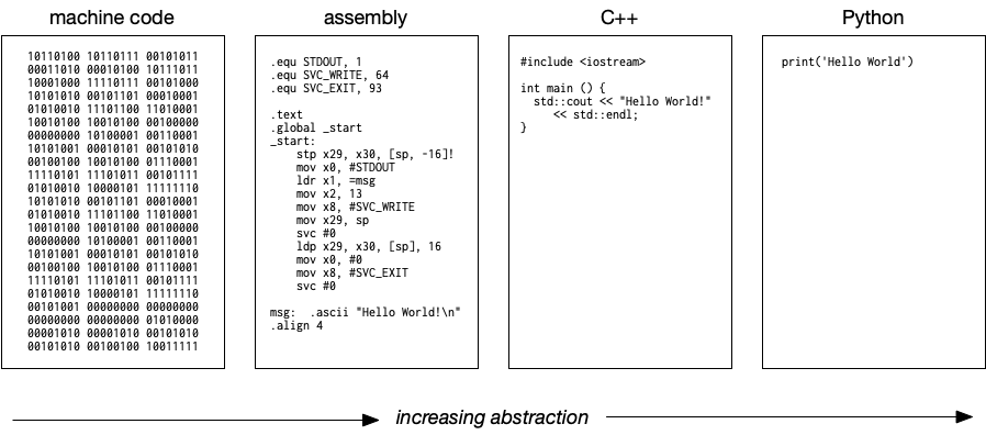
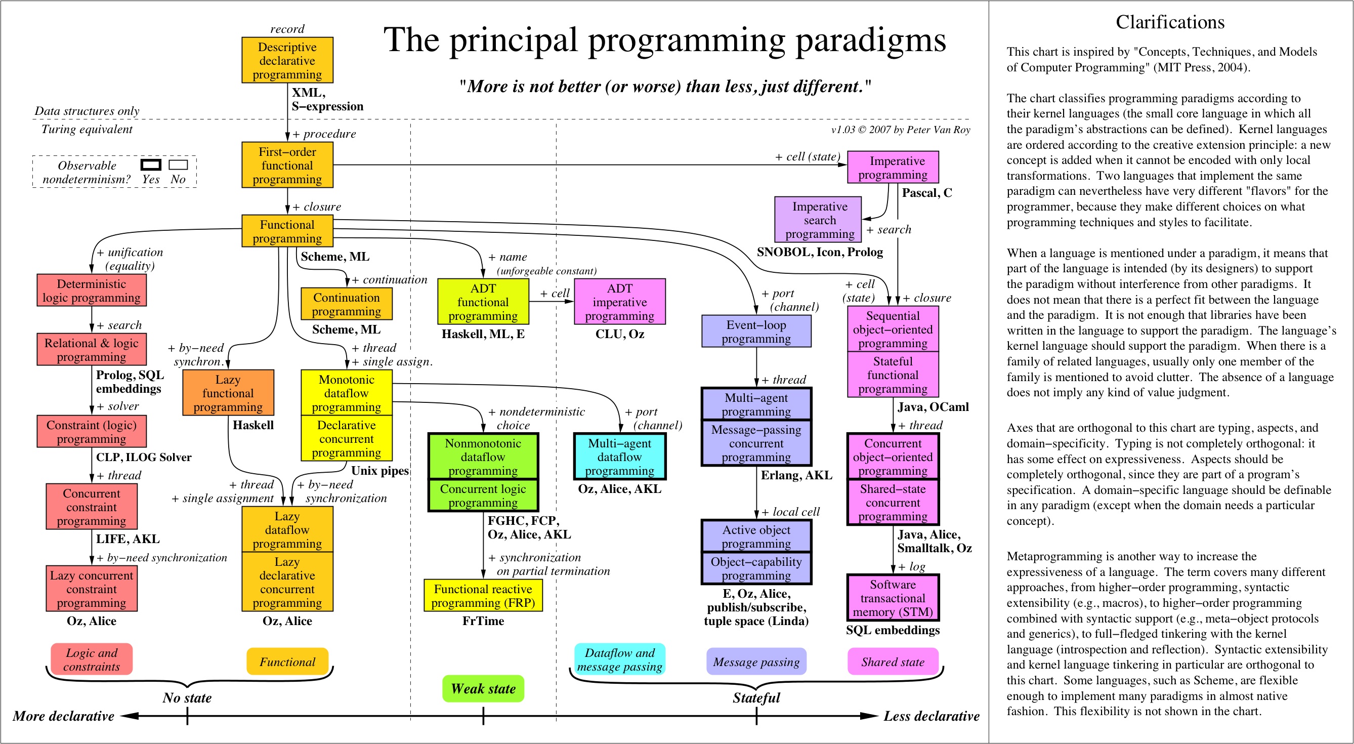
Programming paradigms imposed discipline on program structures. Structured programming (Dijkstra, 1968) restricted control flow to sequence, selection, and iteration, which the Böhm-Jacopini theorem (1966) had proved sufficient for any flowchart program. Object-oriented programming (Simula, 1967; Smalltalk, 1980) organised programs around objects hiding state behind interfaces. Functional programming (lambda calculus, 1936; Lisp, 1958) favoured pure functions and immutable data which became useful for concurrency. Apparently, PL designers shape syntax, type systems, and std. libraries around a preferred paradigm, though most features serve several.
For instance, every language must fix its scoping rule, which determines where a binding is visible. Dynamic scoping resolves a variable to the most recent binding on the call stack, whereas lexical scoping (ALGOL 60, 1960; Scheme, 1975) resolves by position in the source text, so a function sees the environment in which it was defined. In turn, nearly all modern languages adopted the latter for predictable reasoning, each with its own lookup order (e.g. Python’s LEGB: Local, Enclosing, Global, Built-in). Combined with first-class functions, lexical scoping yields closures, which then underpin callbacks, decorators, and also stateful higher-order functions (PEP 227, PEP 318).
-
Van Roy's map of the principal paradigms, each reached from another by adding one concept.
1.2. Type System
A bit pattern means nothing until given a type. The byte 01100001 is the integer 97 under arithmetic (e.g. $+, \times$) or the character ‘a’ under concatenation (per ASCII/Unicode). A data type is the tag that supplies missing context, a domain of values and the operations permitted on them, and the type system comprises a PL’s rules for assigning and checking these types. Concretely, primitive types (e.g. int, float, char, bool) have fixed representations, and data structures (e.g. stack, list, tree, hash map) carry invariant-bound internal state that any C code can access (e.g. s.data[50]). Such access silently broke dependents as codebases grew in the 1960s-70s.
As a remedy, Barbara Liskov introduced the abstract data type (ADT, 1974), a specification of operations and invariants (e.g. peek, push, pop preserving LIFO order) independent of implementation and language. Her own CLU (Turing Award, 2008) was the first to enforce it, for its compiler rejects access to a type’s hidden representation. Encapsulation, as it came to be called, further provided i) correctness; ii) modularity; and iii) substitutability (the Liskov Substitution Principle, 1987). Modern languages inherit that compiler-enforced access control (e.g. Java, Rust), dynamic languages enforce only at runtime (e.g. Ruby), while Python’s _ prefix is convention, not enforcement.
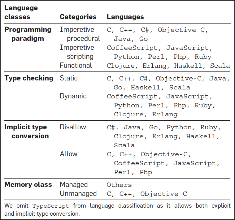
A violation is an operation outside a type’s domain, and PLs differ in when their type system detects one (i.e. type discipline). Statically-typed languages catch them before the program runs, whereas dynamically-typed ones check values as execution reaches them. Even Java, statically typed, defers array bounds to runtime. On the other hand, strong typing rejects implicit coercion (e.g. 2 + ‘2’ raises TypeError in Python), while weak typing permits it (e.g. 2 + ‘2’ yields ‘22’ in JavaScript, and C silently truncates int x = 3.14 to 3 despite its static checks). Both axes decide where a PL’s bugs surface, at compile time, at runtime, or never.
Static typing was safe but verbose. Robin Milner (Turing Award, 1991) dissolved the tradeoff using Hindley-Milner (HM) type inference in Meta Language (ML), where let f(x) = x + 1 compiles to $f : \text{int} \to \text{int}$ without annotations. HM works because each use of a value constrains its type variable, and unification solves for the principal type (Damas and Milner, 1982). It enabled Haskell and influenced Rust, Swift, and Kotlin. Gradual typing (Siek and Taha, 2006) took the opposite path, retrofitting optional annotations as implemented in Python’s type hints (PEP 484), checked by external tools (e.g. mypy, pyright) but ignored at CPython runtime, e.g. def f(x: int) -> int.
-
Languages classified by paradigm, checking time, implicit conversion, and memory management.
In the terms of abstract algebra, an ADT is an algebraic structure $(S, {o_i}, \mathcal{A})$. Its domain, operations, and invariants are respectively the carrier set $S$, family ${o_i}$, and axioms $\mathcal{A}$. While the ADJ group at IBM made this reading exact via initial-algebra semantics (Goguen et al., 1977), the field studies what is deducible from the axioms alone, so a theorem proved once holds in every structure satisfying them. One such theorem, the uniqueness of inverses, can be applied to any group as $(\mathbb{Z}, +)$, $(S_n, \circ)$, and $(GL_n(\mathbb{R}), \times)$. Both group and stack thus fix their axioms and leave the carrier free. That freedom buys programming both equational reasoning and generic code.
The parallel extends even to what an operation excludes. $\sqrt{-1}$ is undefined in $\mathbb{R}$, .append() is undefined on an integer, and each system rejects rather than guesses. Yet the parallel breaks at extension and membership. Unlike mathematics, which chains its number systems $\mathbb{N} \subset \mathbb{Z} \subset \mathbb{Q} \subset \mathbb{R} \subset \mathbb{C}$ to admit new solutions (e.g. $x + 3 = 1$ in $\mathbb{Z}$, $x^2 = -1$ in $\mathbb{C}$), types form a lattice rather than a chain (e.g. numbers, lists, trees). In membership, $3 \in \mathbb{Z}$ and $3 \in \mathbb{R}$ are the same object, while int 3 (0x00000003) and float 3.0 (0x40400000) are in distinct hexadecimal. Therefore, the embedding $\mathbb{Z} \hookrightarrow \mathbb{R}$ costs maths a single act of identification but a program pays a conversion instruction.
Implementations realise these specifications under finite hardware, exactly or approximately. int32 realises the quotient ring $\mathbb{Z}/2^{32}\mathbb{Z}$ exactly, for wrapping arithmetic is reduction mod $2^{32}$, and approximates the infinite $(\mathbb{Z}, +, \times)$ using the representatives $[-2^{31}, 2^{31}-1]$. str approximates a free monoid $(\Sigma^\ast, \cdot, \varepsilon)$ as a byte array bounded by memory. Concatenation is its operation, the empty string $\varepsilon$ its identity, and the monoid is free, i.e. nothing holds beyond the axioms. list approximates the same free monoid over a type $T$, $(T^\ast, \cdot, [])$, and list[str] is then $\Sigma^{\ast\ast}$ , the construction applied twice. Whatever storage and algorithms realise them remain details the ADT hides.
-
Structure Ops Axioms Example What works What doesn't monoid one associativity, identity $(\mathbb{N}, +)$, $(\mathbb{N}, \max)$ $3 + 5 = 8$, $\max(3,5) = 5$ $(-5) \notin \mathbb{N}$, no inverse for $\max$ group one monoid + inverses $(\mathbb{Z}, +)$ $8 + (-5) = 3$ — ring two additive group, multiplicative monoid, distributivity $(\mathbb{Z}, +, \times)$ $3 \times 5 = 15$ $5^{-1} \notin \mathbb{Z}$ field two ring + commutativity + multiplicative inverses $(\mathbb{R}, +, \times)$ $5x = 3 \Rightarrow x = 3 \cdot 5^{-1}$ — vector space two abelian group $(V,+)$ + scalar mult. from field $F$ $(\mathbb{R}^n, +, \cdot)$ $\vec{u} + \vec{v}$, $\alpha \vec{u}$ no vector $\times$ vector Hilbert space three vector space + inner product + completeness (topological, not equational) $(L^2, +, \cdot, \langle\cdot,\cdot\rangle)$ $\langle f, g \rangle = \int f \bar{g}$ —
Types also compose in the terms of set theory. A struct or tuple is a Cartesian product ($\text{String} \times \text{Int} = \Sigma^\ast \times \mathbb{Z}$), a tagged union or enum is a disjoint union (Rust’s $\text{Result}\langle T, E \rangle = T \sqcup E$), and a function type $A \to B$ has $\vert B\vert ^{\vert A\vert }$ inhabitants for finite $A$, $B$. These are known as algebraic data types because their cardinalities follow arithmetic ($\vert A \times B\vert = \vert A\vert \cdot \vert B\vert $, $\vert A \sqcup B\vert = \vert A\vert + \vert B\vert $), and the arithmetic predicts real counts. $\text{Bool} \to \text{Bool}$ has exactly $2^2 = 4$ inhabitants (identity, negation, constant true, constant false), and $\text{Option}\langle T \rangle = T \sqcup 1$ has $\vert T\vert + 1$ values, the extra one being None. Type constructors like List go further as functors $\textbf{Type} \to \textbf{Type}$, lifting a function $f : A \to B$ to $\text{map}(f) : A^\ast \to B^\ast$ while preserving composition.
Under the Curry-Howard correspondence (Curry, 1934; Howard, 1969), the same constructions read in the terms of mathematical logic. A type is a proposition and its inhabitant is a proof, hence $A \times B$ is conjunction (evidence of both), $A \sqcup B$ is disjunction, and $A \to B$ is implication, where a function claims to construct evidence of $B$ from evidence of $A$ and its body is the proof. The empty type admits no inhabitants and so no proofs, which makes it falsehood. Type-checking thereby becomes proof-checking, and Lean and Coq exploit it as theorem provers. A theorem is stated as a type, its proof is a program of that type, and the compiler checks the given proof mechanically.
-
Mathematics CS Object element of a set ($3 \in \mathbb{Z}$, $f \in L^p$) bit pattern with a type label Structure carrier + operations + axioms (e.g. group, field) ADT: carrier + signature (e.g. int, list) Implementation — data structure (e.g. hash map, BST) Context implicit (mathematician tracks it) explicit (type annotation or inference) Composition $A \times B$, $A \sqcup B$, $A \to B$ product, sum, function types Cardinality infinite ($\vert\mathbb{Z}\vert = \aleph_0$) finite (int32 has $2^{32}$ values) Verification peer review, proof type checker, compiler
1.3. Memory Management
Every object a program allocates occupies memory for its lifetime, and memory being finite, a program that never reclaims memory for reuse will exhaust it. Static allocation, as in Fortran, left nothing to reclaim, sizes fixed at compile time and slots held for the whole run. Dynamic data arrived with Lisp’s heap allocation for objects of unknown size/lifetime (§603#3.1). While it reclaimed the heap automatically via garbage collection (GC), C (1972) left it to the programmer through malloc/free from its std. library. In practice, manual discipline failed at scale, as Microsoft (MSRC, 2019) and Chromium (2020) each attribute ~70% of their C/C++ vulnerabilities to memory bugs.
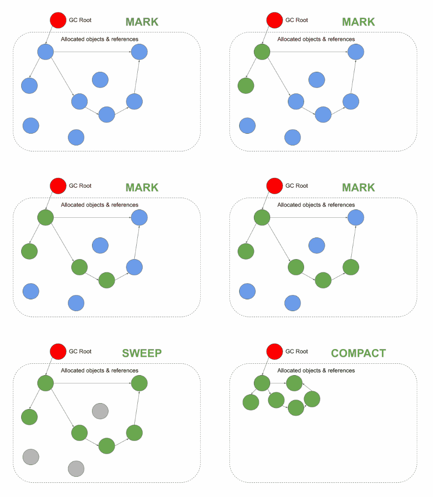
How a collector finds garbage splits GC into three forms: i) reference counting (e.g. CPython): each object carries a count and is freed the moment it drops to zero, though cycles keep counts positive; ii) mark-and-sweep: the collector traces reachable objects from roots (e.g. globals, stack variables) and frees the rest, which classically stops the world, though incremental and concurrent variants run tri-colour marking alongside the program to keep each pause short; and iii) generational collection (e.g. Java, .NET): most objects die young, thus the youngest generation is collected most often. All three conveniently automate reclamation at the cost of non-deterministic pauses.
CPython stakes reclamation on that reference counting, while the cyclic collector (the gc module) backstops cycles. The counts free memory promptly and deterministically, while C extensions must balance Py_INCREF/Py_DECREF by hand. Given that a simple read also mutates the count (i.e. ob_refcnt), the GIL (§604#2.3) guards these writes, and the free-threaded build makes the counts atomic and locks per object instead. In practice, del merely unbinds a name and decrements, and an object is freed only when its last reference goes (e.g. a NumPy view pins its base array). A forked worker loses its copy-on-write pages just by reading (§603#3.1).
How much type information a PL preserves at runtime shapes what it heap-allocates, what it automates, and what each value costs. C, a statically-typed language, erases types after compilation and places local variables on the stack as raw bits (e.g. int, 4 bytes), reclaimed manually. Java, also statically-typed, heap-allocates its objects (e.g. Integer, ~16 bytes; GC-managed) but stack-allocates primitives (e.g. int, 4 bytes). Python, dynamically-typed, binds type information to every value as a heap-allocated PyObject (e.g. int, ~28 bytes) carrying metadata (reference count, type pointer) beside the payload. Each buys automation with bytes per value.
-
Mark-and-sweep tracing reachable objects from the GC root before sweeping the rest.
1.4. Error Handling
An error is a condition preventing a call from producing its desired result, and every such call must report back to its caller. In practice, the failures differ in where the report is lost, i) the caller: C, for instance, signals failure with a sentinel value (-1, NULL) and errno that one unchecked return silently discards; ii) the PL: Tony Hoare’s null reference (ALGOL W, 1965), a “billion-dollar mistake” in his words, inhabits every reference type and turns every dereference into a latent error; and iii) the context: Ariane 5 (1996, $370M) inherited code from Ariane 4, and a conversion that could never overflow on the old rocket did on the new one. All three fail far from the code at fault.
C’s successors traded between two goods, a clean happy path and visible failure. Exceptions (PL/I, 1964, ON-conditions; formalised in CLU, 1979) chose cleanliness, unwinding the call stack to a matching handler while hiding the set of possible failures from the signature. Go (2009) chose visibility, returning to explicit error codes that expose failure at every call site (if err != nil). Algebraic error types such as Haskell’s Either and Rust’s Result$\langle$T, E$\rangle$ reconcile the two by encoding success or failure in the type, hence the programmer must handle or propagate it and the compiler warns when a Result is discarded.
Yet not every error deserves handling. A bug is a defect in the program itself, whereas a recoverable condition (e.g. a missing file) is still an error but one arising from the outside world. The test is whether it could befall a correct program, hence a contract violation (e.g. an index out of bounds) signals a bug beyond local repair. Python, specifically, marks the divide in its exception hierarchy, where handlers catch Exception to recover, while BaseException subclasses (e.g. KeyboardInterrupt) terminate the run. Furthermore, Python’s EAFP idiom treats recoverable errors as ordinary control flow, trying the operation and catching what fails rather than checking beforehand.
II
2.1. Compiler
A compiler is a program that batch-translates source code into a lower-level language, often assembly or machine code, before execution. While Von Neumann reportedly dismissed even an assembler as a clerical waste of a scientific device, Grace Hopper’s A-0 system (1952), the first so-called compiler, mapped mathematical notation to pre-written subroutines. Five years later, Fortran settled the argument with machine code that rivalled hand-written assembly. Theory then caught up, as the Chomsky hierarchy (1956) classified grammars by expressive power, Backus-Naur form (BNF, 1959) gave them a notation, and Lex and Yacc (1975) automated lexer and parser generation.
These formalisms underpin the first stage of the standard compilation pipeline. Specifically, the front-end carries out i) lexical analysis: breaks source code into tokens; ii) parsing: builds an abstract syntax tree (AST); iii) semantic analysis: checks types and resolves scopes; and iv) intermediate representation (IR) generation. The middle-end optimises the resulting IR (e.g. constant folding and propagation, dead-code elimination, inlining) through static single assignment (SSA) form. The back-end finally lowers the optimised IR to machine code for a target ISA, while a linker combines object files (e.g. .o, .obj) into an executable bound to a specific OS and ISA.
This division of labour has evolved over generations of compilers. For example, early compilers were monolithic, built for one language on one target. The GNU Compiler Collection (GCC, 1987), the first major free compiler, proved that a single codebase could serve many languages and target ISAs. GCC is moreover self-hosting in that it compiles its own source through bootstrapping. However, its IRs (i.e. GENERIC, GIMPLE, RTL) stayed internal and unstable. Each front-end was therefore written against GCC’s shifting internals instead of a stable interface, and supporting $N$ languages on $M$ targets meant wiring every language-target pair, an effort proportional to $N \times M$.
-
The front-end and middle-end feeding target-dependent back-end stages, with the assembler and linker outside the compiler proper.
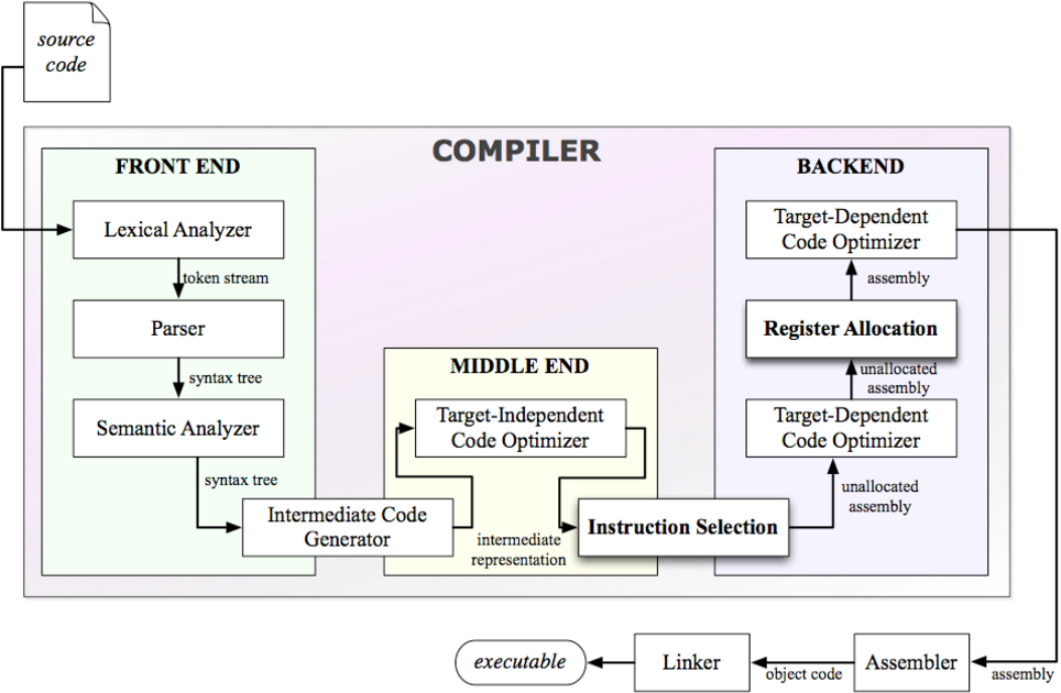
Low-level virtual machine (LLVM, 2003), begun as Chris Lattner’s graduate project at the University of Illinois, collapsed the product to the sum $N + M$ by defining a stable, target-independent IR in SSA form (textual .ll, binary .bc). The pattern is general, for wiring both sides of such a dependency to a shared hub requires only $N + M$, an argument that recurs for editor-language and agent-tool protocols (§605#4.4). The developer’s dividend is that the task reduces to emitting correct LLVM IR since optimisation and code generation come free. A new ISA’s dividend is symmetric in that one back-end shared by every language replaces a change to each compiler.
-
Three front-ends and three back-ends meeting at one optimiser over LLVM IR.
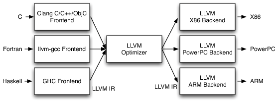
Both dividends played out first in C’s own toolchain. LLVM initially relied on GCC as its front-end (llvm-gcc) until Clang (2007) replaced it with a native C/C++/Objective-C front-end. The shared middle-end and back-ends indeed stayed untouched, while the one IR Clang emits lowers to any supported ISA, which the back-end can compile ahead-of-time (AOT) via llc or execute just-in-time (JIT) via lli. A flag moreover pauses the pipeline after any stage of compilation and exposes its output. For example, the preprocessor expands macros and #includes (-E), the compiler emits assembly (-S), the assembler produces an object file (-c), and a full run carries on through linking.
-
The Clang front-end feeding LLVM's shared middle-end and back-ends.

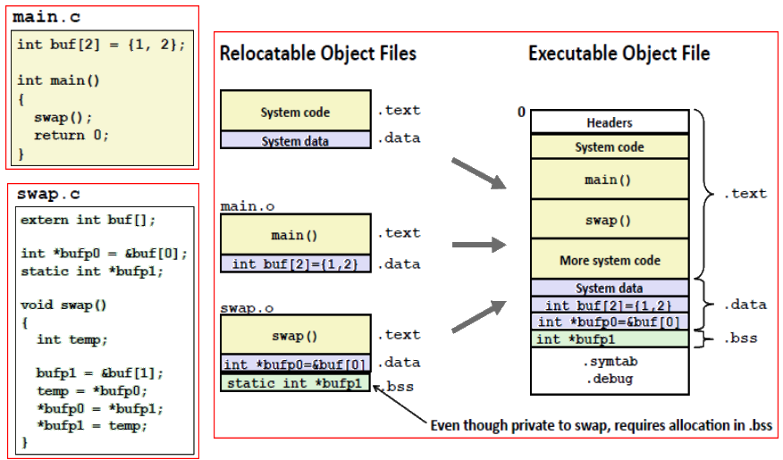
The linker combines object files, potentially from different source languages, but the result is correct only if all were compiled against the same application binary interface (ABI), which specifies calling conventions, data type sizes, struct layout, and name mangling. To combine, the linker resolves each file’s references to symbols the others define and relocates their sections to final addresses. Static linking embeds all dependencies into the executable, while dynamic linking defers resolution to shared libraries (e.g. .so, .dylib) at load time via a runtime linker (ld.so on Linux, dyld on macOS). An ABI mismatch may silently corrupt data or crash at runtime.
The finished binary is the program itself, its sequence of instructions now bound to a triple $(\text{ISA}, \text{vendor}, \text{OS})$, thus running it elsewhere needs translation. Apple’s Rosetta 2, for instance, bridges the ISA mismatch by rewriting x86_64 binaries for ARM (i.e. AOT as default, JIT as a fallback). The OS field then decides the on-disk format. Linux, Windows, and macOS define the executable and linkable format (ELF), the portable executable (PE), and Mach-O, respectively. Each lays out machine code and data as segments behind a header that the OS loader reads to map the executable into memory, and a process is the executable image extended with a heap and a stack (§603#3.1).
Therefore, the executable holds more than the machine code the compiler emits, as its header also records the entry point and the shared libraries the runtime linker must supply. The first bytes form the magic bytes (aka. file signature), 0x7F ‘E’ ‘L’ ‘F’ for ELF, and exec() dispatches on them, so a #! opening routes a script to its interpreter instead. The kernel never consults the file name, so extensions on Unix remain a user-space convention, and the file utility likewise identifies content by signature. Data files follow the same convention (e.g. %PDF, Parquet’s PAR1), as bytes on disk, like bit patterns in memory, mean nothing until tagged.
-
Two relocatable object files merging section by section into one executable, headers in front.
2.2. Domain-Specific Compiler
A general-purpose language (GPL) commits to no particular domain. A domain-specific language (DSL) confines its abstractions to one and encodes domain knowledge as primitives that a GPL must reconstruct by loops, conditionals, and data structures. A GPL compiler that emits standalone machine code, yet each DSL is backed by its own compiler or interpreter, and a compiler targets its own executor (e.g. DB engine, regex engine, GPU runtime). For instance, a structured query language (SQL) offers grouping (GROUP BY) and aggregation (AVG) as primitives, and the query processor in DB compiles such a declarative query into a physical execution plan (§606#3.2).
Note that confining the language is what licenses guarantees a GPL compiler cannot make. For example, a regular expression (regex) is a language sufficiently restricted that any pattern compiles into a finite automaton, whose execution costs one step per character. Google’s RE2 (2010) rests on this bound and matches in linear time, whereas backtracking engines (e.g. Python’s re) admit an exponential worst case exploitable as a denial of service (ReDoS). SQL enjoys the same freedom. A rewrite such as join reordering is a universal theorem of relational algebra valid for all queries, while a compiler given the same query as loops must prove each transformation safe per program.
While SQL and regex stand alone with their own grammar, an embedded DSL resides inside a host GPL and borrows the host’s toolchain and, typically, its syntax yet keeps its own compiler. The embedding takes several forms, i) operator overloading: df.filter(df[“age”] > 21) in PySpark redefines > to build a query plan optimised by Catalyst rather than a boolean; ii) decorated functions: a GPU kernel marked @triton.jit is compiled outside the Python interpreter; and iii) pattern strings: even regex often appears embedded, passed to re.findall. Residence is thus a property of use, not of the language, as the same pattern grammar serves grep standalone and Python embedded.
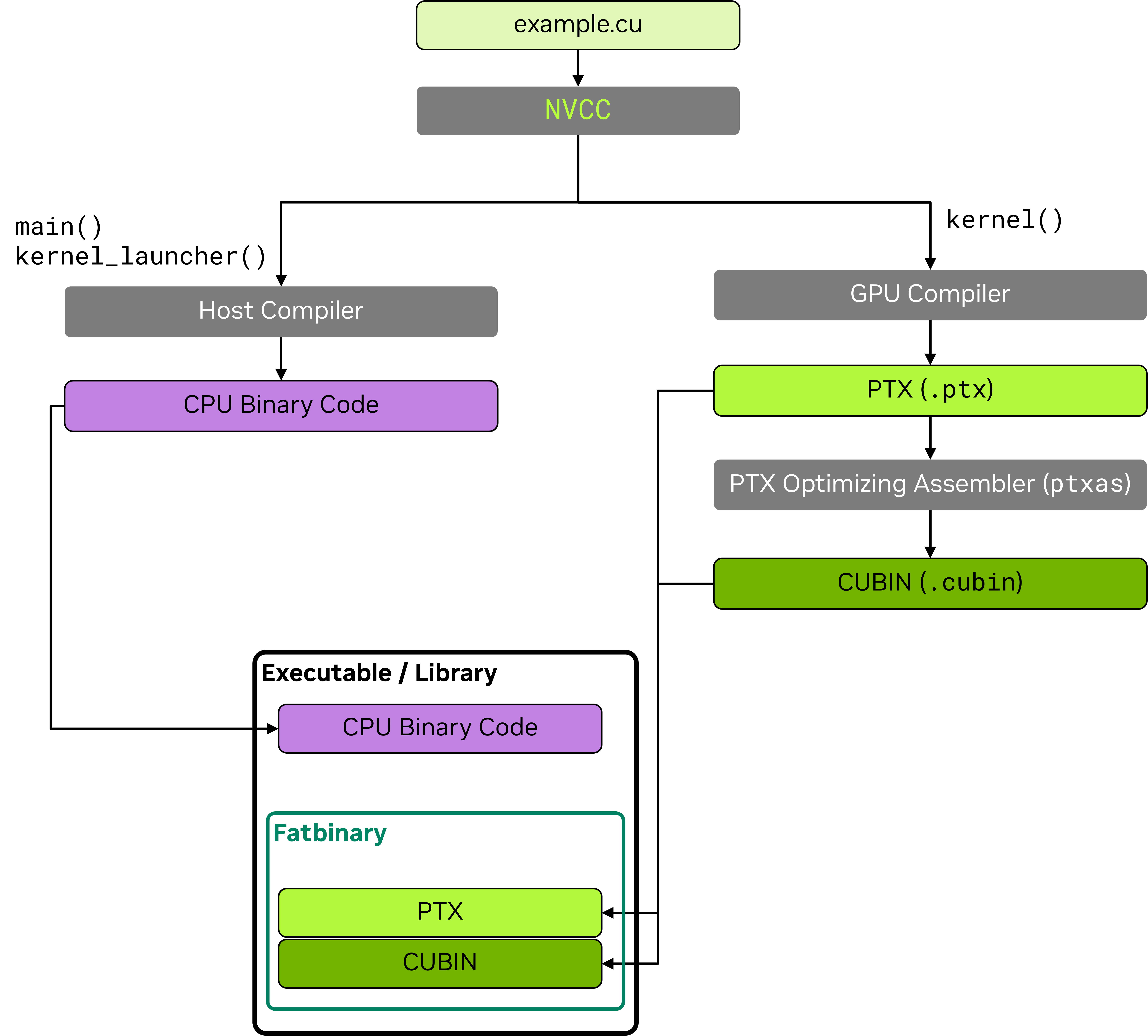
In the ML era, a flagship embedded DSL is Compute unified device architecture (CUDA), extending C/C++ with GPU-specific constructs for programming NVIDIA hardware (§601#2.1). Its dedicated NVIDIA CUDA compiler (NVCC) breaks source code from a .cu file into device code (i.e. kernels marked with __global__/__device__) and host code (i.e. CPU logic), translates the former through NVIDIA’s LLVM derivative (NVVM) to parallel thread execution assembly (.ptx) or a directly executable CUDA binary (.cubin), and delegates the rest to the host compiler. For example, a kernel launch add«<grid, block»>(args) is invalid C++ until NVCC rewrites it into runtime API calls.
-
NVCC splitting a .cu file, host code to the host compiler and kernels through ptxas into a fatbinary (simplified to one architecture).
DSLs long paid the price of a full toolchain built from scratch as CUDA did. GPL compilers had already escaped this cost by sharing the LLVM hub, but the hub covers only the bottom half of the compilation pipeline, which lowers unoptimised IR down to machine code, and yields little for a DSL whose value lives above the IR. For instance, a lowered tensor operation is mere loop nests of scalar arithmetic with no record that they constitute a matmul, hence fusing two such operations into one kernel is intractable. Consequently, each project rebuilt its own middle layer (e.g. Swift-SIL, Rust-MIR, TorchScript) above LLVM IR and duplicated passes, lowering, and verification.
Chris Lattner repeated the consolidation one level higher with the multi-level intermediate representation (MLIR) at Google in 2019. It introduced the dialect (i.e. a domain’s operations and types) and supplies the shared infrastructure (passes, verification, rewriting) along the way down to LLVM IR. Built-in dialects (arith, linalg, gpu) are maintained by the LLVM community. External projects make their own (e.g. torch-mlir, IREE). A PyTorch tensor addition lowers from torch.aten.add (Torch dialect) to element-wise loops (linalg.generic) to scalar arithmetic (llvm.fadd). In sum, LLVM standardised everything below the IR, and MLIR standardises everything above it.
Triton (OpenAI, 2021), once Philippe Tillet’s PhD project, is a Python DSL for GPU tensor operations built on MLIR, which evidence that a DSL now costs only its dialect. It automates what CUDA leaves manual (i.e. coalescing, synchronisation, SM scheduling) by replacing the per-thread SIMT model with tile-based programming. Its compiler captures the kernel’s AST and lowers it dialect-by-dialect: Triton IR (TTIR, hardware-agnostic) → TritonGPU IR (TTGIR, hardware-specific) → LLVM IR → executable. Triton sits between eager-mode PyTorch (no kernel control) and raw CUDA (full manual control) and exposes shared memory and HBM but not thread-level scheduling.
-
MLIR's dialects filling the abstraction gap between the AST and LLVM IR.

III
3.1. Interpreter
A compiler buys maximum runtime speed ahead of time, whereas an interpreter executes source-level representations without producing a standalone binary, trading speed for immediacy and portability. The approach began unintentionally when eval, a Lisp function that evaluates any Lisp program, appeared as pure theory in an ACM paper (McCarthy, 1960). His student Steve Russell then hand-translated it into IBM 704 machine code, yielding the first Lisp interpreter and in time the read-eval-print loop (REPL). Interpreters enable runtime dynamism (e.g. eval(“2+3”), getattr(obj, “method”)) which a standalone AOT binary supports only by bundling an interpreter of its own.
The Unix shell (1971, §603#2.2) had meanwhile made an interpreter every programmer’s front door to the OS, a REPL whose expressions are commands. Interpreters then carried programming into the home, where Altair BASIC (1975) launched Microsoft and late-70s machines booted straight into a ROM BASIC as their sole interface. The REPL’s modern face is the Jupyter notebook, grown from physics graduate student Fernando Pérez’s IPython (2001). Hardware underwrote each step, as timesharing first made computing conversational and every generation of Moore’s law shrank the interpreter’s constant-factor penalty against the programmer hours it saved (Ousterhout, 1998).
What an interpreter re-executes is a representation, thus the choice sets the speed. Early interpreters tree-walked, re-traversing the AST with per-node pointer chasing on every run. A bytecode interpreter instead splits the work in two, i) compilation: the tree (e.g. ast.parse) is flattened once into an instruction array; and ii) execution: one loop dispatches each instruction to its handler. Reading a pre-decoded instruction like LOAD_FAST 0 (i.e. push local variable slot 0) is clearly cheaper than re-deriving a node’s meaning at every visit. Locality also favours bytecode because consecutive instructions share a cache line while each AST pointer may land on a cold one.
The shell and R’s default evaluator remain tree-walkers since code run once gains nothing from flattening. Bytecode by contrast requires an executor of its own. As machine code is bound to a specific ISA, bytecode is bound to a specific virtual machine (VM), a machine made of software rather than silicon. A system VM implements the full computer (§607#1.1), whereas an interpreter uses a process VM that implements only a CPU, whose invented ISA (e.g. BUILD_LIST) exists in no silicon. The process VM is thus an ordinary user process that executes natively, delegates everything physical (memory, I/O) to its host OS, and compiles for any platform, which earns bytecode its portability.
The model is older than its slogan. UCSD Pascal (1978) already compiled to p-code that a small interpreter ran on any machine, 17 years before Sun sold the JVM as write once, run anywhere. Java (1995) popularised it with its Java virtual machine (JVM) that became a compilation target of other languages (e.g. Scala, 2004). Stack-based VMs (e.g. JVM, CPython) push and pop operands on an implicit stack, which keeps each instruction tiny and the compiler simple, whereas register-based VMs name operand locations in each instruction and so need fewer of them. Lua switched from the former to the latter at 5.0 (2003), judging fewer dispatches worth the fatter encoding.
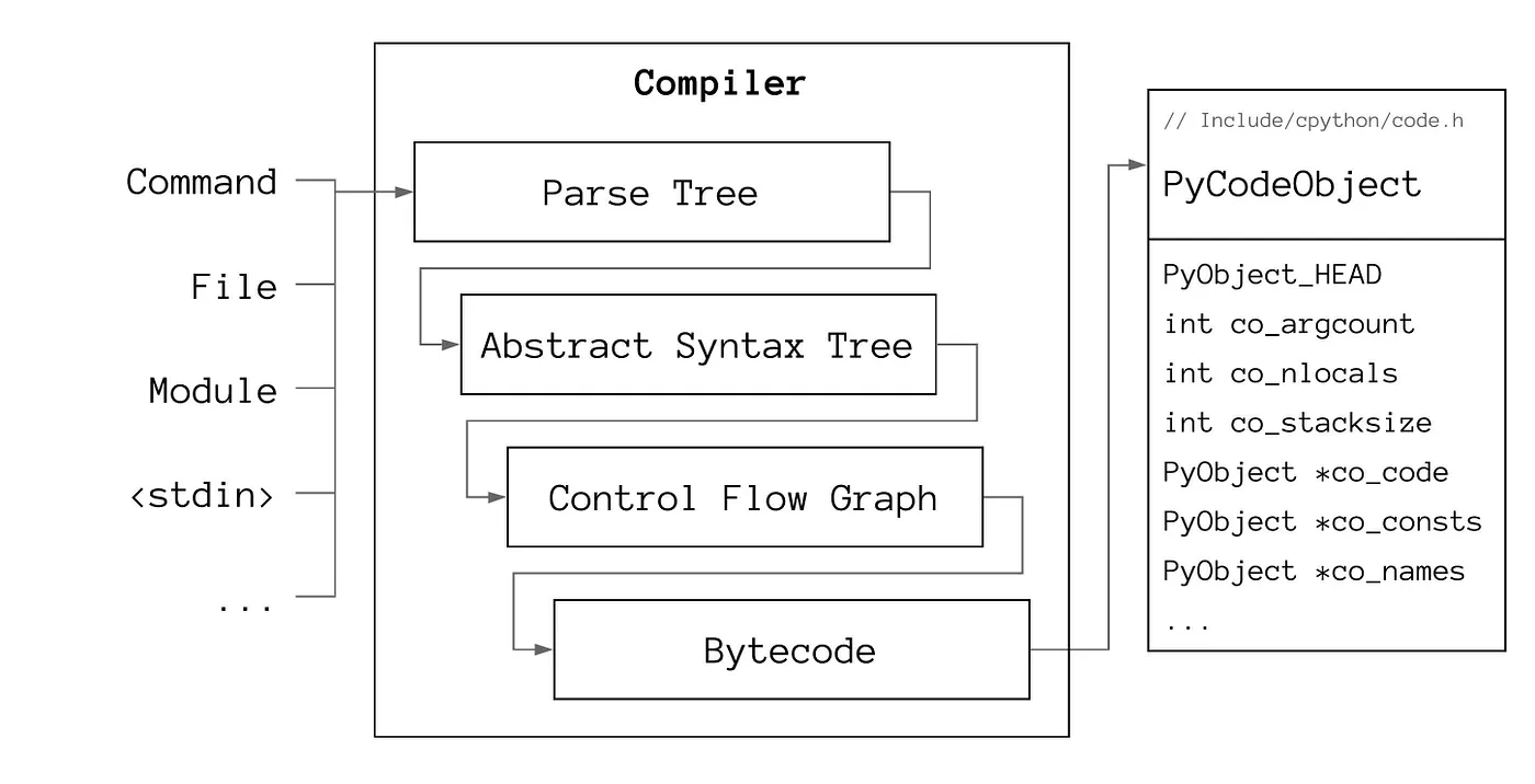
In particular, CPython (1991) by Guido van Rossum is a compiled C binary of the two halves, a compiler that turns source into bytecode held in code objects and a PVM for its execution. The bytecode consists of operation codes (opcodes) paired with operands, each similar to an assembly mnemonic (e.g. LOAD_FAST, BINARY_ADD) whose operand indexes into the code object’s tables (e.g. the dis module disassembles bytecode into this readable form). The compiled code objects are also serialised (§605#4.1) as __pycache__/*.pyc (PEP 3147), and this disk cache spares recompilation between runs, until the source changes or the header’s magic number names another release.
-
The interpreter's two halves, a compiler emitting bytecode and a PVM executing it.
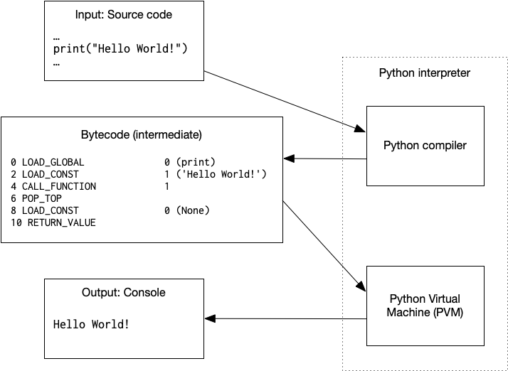
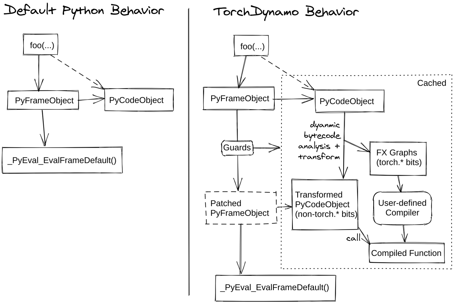
In the C source, the compilation entry point (i.e. _PyAST_Compile in Python/compile.c) transforms the AST into a PyCodeObject, which encapsulates the bytecode (co_code) with its tables (i.e. constants, names, closures). The PVM, C functions linked into that same binary, executes it in a dispatch loop (i.e. _PyEval_EvalFrameDefault in Python/ceval.c, the evaluator in C, still named for eval), an ordinary C function behind a swappable pointer (PEP 523). Each iteration fetches one opcode, decodes its operand, and jumps to the C handler that performs it, the fetch-decode-execute cycle (§601#1.2) rendered in software. Note that the GIL lets a single thread into this loop at a time.
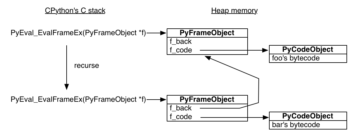
C pins machine code in the text segment and per-call state in a stack frame popped at return. CPython instead puts code object, function object, and frame all on the heap managed by GC. The frame is the call’s workspace, its locals and operand stack (localsplus), linked to its caller (f_back) in the chain the traceback prints. On this ground stand the stateful functions. The function object is the first-class value and the surviving frame is the captured environment, which closures, generators (PEP 255, 2001), and coroutines (PEP 492, 2015) build on. For instance, a suspended generator keeps its frame frozen at the yield, which may be seen as a user-space context switch (§604#1.3).
The adaptive interpreter (PEP 659) specialises hot opcodes (e.g. BINARY_OP → BINARY_OP_ADD_INT) but does not close the dispatch gap for compute-heavy workloads. Performance-critical Python instead bypasses the interpreter through C extensions, as NumPy delegates linear algebra to BLAS/LAPACK, PyTorch dispatches to CUDA kernels, and the standard library itself wraps C implementations (e.g. json, re). The bindings come via CPython’s C API, Cython, or pybind11, and the shipped wheels must match the interpreter’s ABI unless built to the stable ABI (abi3, PEP 384). Python orchestrates while heavy computation runs at native speed, which is why it dominates ML and scientific computing.
-
Each call links a heap PyFrameObject to its caller via f_back while the C stack recurses.
3.2. Just-In-Time Compilation
Just-in-time (JIT) compilation translates the running program into machine instructions, pairing the interpreter schedule with the AOT compiler output. Specifically, the runtime profiles execution to identify the frequently executed regions (i.e. hot spots), and also restricts compilation to the small fraction of the codebase that dominates the running time, as the 90/10 rule measured by Knuth (1971) on the FORTRAN programs. Compilation is deferred into the run because only the executed program reveals where the hot spots lie. Ideally, the hybrid achieves interpret-less speed at compile-less overhead, nearing what those extensions deliver without their rewriting effort.
A JIT compiler arbitrates the pull between interpret-less and compile-less by counting function and loop executions. It compiles a region over the threshold, patches its call site, and later calls skip the interpreter. Observed runtime types enable speculative optimisations an AOT compiler cannot make and deoptimisation reverses them when an assumption fails. Production runtimes further stack tiers from a fast baseline to a slower optimiser and promote a region upward as its count rises. Runtime compilation predates its name, from QED (Ken Thompson, 1968) compiling regular expressions mid-run up to CPython gaining a JIT in 3.13 (2024) under the Guido van Rossum.
The same pull recurs in the deep learning frameworks, TensorFlow (Google, 2015) and PyTorch (Facebook, 2017), where the compilation unit is a tensor program. Each implements the program’s two primitives, the tensor, an order-$n$ array of the coordinates of a multilinear object in fixed bases, and differentiable operations on tensors (e.g. matrix multiplication). A neural network amounts to a composition $f_\theta = f_k \circ \cdots \circ f_1$ of those operations, and trained by gradient-based optimiser whose every step requires $\partial J/\partial \theta_i$ of the objective $J$ w.r.t. each parameter $\theta_i$. Both frameworks build a graph to backpropagate the gradients but differ in when it is formed and how it is executed.
PyTorch adopted define-by-run (i.e. eager execution) and forms a dynamic computation graph (DCG) as the model runs. Each operation dispatches its kernel on its Python line, and hence debuggers, print, and native control flow apply unchanged. TensorFlow committed to define-and-run (i.e. graph execution) where the user constructs a static computation graph (SCG) and executes it in a session. The SCG is therefore optimisable and exportable whole before it runs. While research widely embraced eager execution (Paszke et al., 2019), even TF 2.0 (2019) made it the default, and the easier graph had quietly lost to the easier code, a verdict the compiler would reopen.
-
A single multiplication recorded, where the output's grad_fn reaches the backward node whose next_functions route the gradient to the leaf that requires it. See PyTorch internals (Yang, 2019).
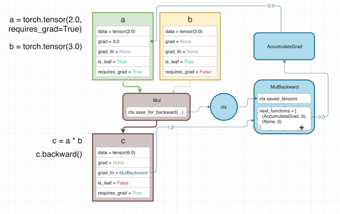
Yet eager’s DCG is built solely for the $\partial J/\partial \theta_i$ and survives a single forward-backward pass. Specifically, Autograd records each operation on a torch.Tensor with requires_grad=True into a graph of torch.autograd.Function objects rooted at the output’s grad_fn, such that .backward() traverses it in reverse (reverse-mode automatic differentiation). Reverse suits a network mapping many parameters to one scalar objective, as one traversal yields every partial derivative. The record is therefore a tape of what executed, rebuilt each forward pass, divergent when a branch differs, discarded once backward consumes it. A compiler is left with no persistent graph to optimise or export.
The transformer architecture (Vaswani et al., 2017) made that persistent graph worth having, the need urgent on three counts and none met by eager’s one precompiled kernel per operation, i) throughput: its elementwise kernels are memory-bound (§601#2.3), as (a + b) * c writes the sum to HBM and reads it straight back for the product, a round trip that only a compiler seeing both can fuse away by keeping the sum in SRAM (He, 2022); ii) deployment: the artefact must carry neither Python nor a GIL which serialises a process’s threads; iii) portability: one graph must retarget to accelerators no hand-written kernel would reach.
Billed as the bridge to production, TorchScript (PyTorch 1.0, 2018) captures the model AOT as a persistent SCG written in TorchScript IR, as torch.jit.trace tapes the path a mock input exercises and torch.jit.script parses the source to preserve control flow. Either serialises to a .pt archive, yet the model as a whole never reaches machine code despite the torch.jit namespace. Execution then falls to LibTorch, PyTorch’s Python-free C++ distribution, whose interpreter walks the graph node by node into the same precompiled kernels, the way CPython walks bytecode. The attempt tackled deployment alone, but rewriting a program into its typed Python dialect cost eager’s ease.
The TorchScript IR it captured is domain-level, just below the source, far above the loop-level and scalar IRs of machine code, and each node names a whole tensor operation that LLVM IR dissolves into scalar arithmetic. It differs from LLVM IR only in its atoms, the form a shared typed SSA graph. The altitude keeps a graph rewrite tractable, as each optimisation applies where its structure is visible, and the middle-end passes followed (e.g. dead-code elimination, constant propagation, a limited NNC fusion of elementwise chains). The descent is one-way, lowering discards structure no pass can recover, and TorchScript’s stopped above the loops, where it sits in maintenance.
-
The 1.x stack twice, its components on the left and one source line descending every altitude on the right.
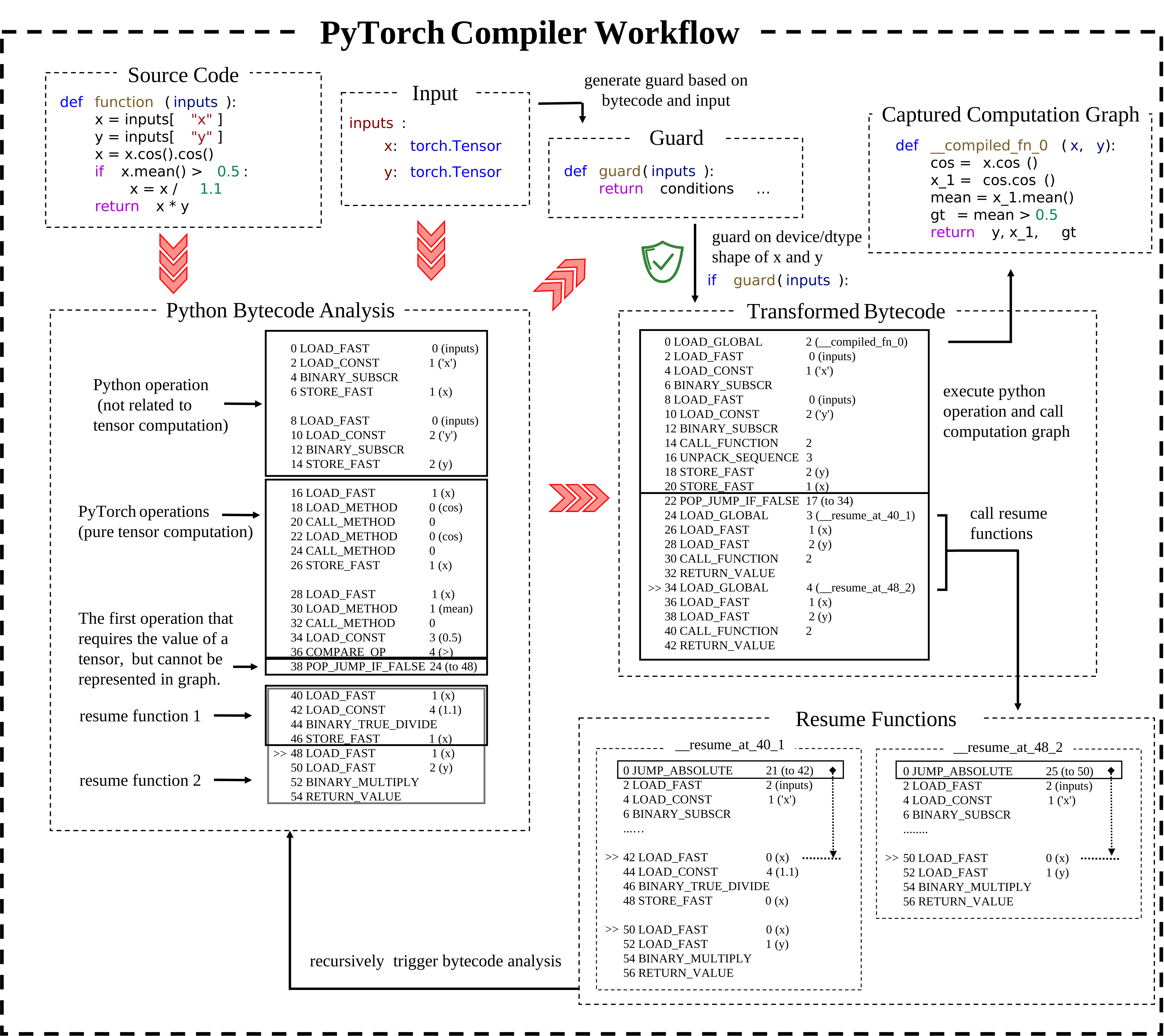
torch.compile (PyTorch 2.0, 2023) moved capture into the run, a tracing JIT comprising front-end, IR, and back-end. TorchDynamo, as front-end, replaces CPython’s frame-evaluation pointer (PEP 523), walks the bytecode, and extracts tensor operations into an FX graph (Reed et al., 2022) in Torch IR. The run produces many guarded subgraphs (i.e. partial SCGs) rather than the one whole graph TorchScript demanded. The SCGs descend through the back-end to machine code, winning the throughput graph-walking never did, for training and inference alike. Nothing need be rewritten, as the untraceable is handed back rather than rejected, eager’s price refunded.
The first bound on the gain is what is visible to the front-end and the same limit leaves the SCGs partial. A graph break arises where the bytecode walk meets Python it cannot trace (e.g. a data-dependent branch, .item()). The break splits the function into subgraphs stitched by resume functions that the plain interpreter runs. torch._dynamo.explain lists each break and its cause, while fullgraph=True turns the silent split into an error. The break costs more than the interpreted stretch itself, since fusion cannot cross the boundary and the live tensors at it must be materialised for the interpreter to hold. A break inside the innermost loop can thus consume the whole gain.
The other bound is what the trace assumed, recorded as guards (e.g. dtypes, shapes) rechecked on every later call. An unseen shape fails its guard and forces a retrace. The second shape is what teaches the compiler because automatic dynamic marks the dimension that moved and retraces it with a symbolic size (SymInt) that later shapes satisfy. Dynamic shapes may instead be declared up front to skip the wasted first pass. The tolerance is finite, since a frame recompiled past cache_size_limit (eight by default) is abandoned to the interpreter permanently, the speculation and deoptimisation of any JIT replayed on tensors.
Past both bounds, an SCG taped from the forward alone enters the back-end. AOTAutograd derives the missing backward, running fake tensors (shapes without data) through eager’s own differentiation rules, and splits the joint trace into forward and backward FX graphs. During the trace, both passes are decomposed into ~250 primitives of ATen, PyTorch’s “A Tensor Library” built in C++ over the vendor kernels of MKL, cuDNN, and cuBLAS. The back-end thus receives the pair in ATen IR, not yet executable and deliberately pessimised (e.g. eager’s fused softmax outruns its separated exp, sum, and divide), but the stable contract between capture and code generation.
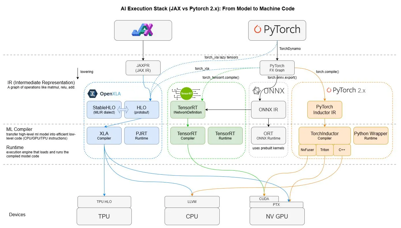
The default back-end TorchInductor lowers the ATen pair into its own loop-level IR to emit Triton for GPUs and C++/OpenMP for CPUs. Each primitive is spelt out over its elements (e.g. the sum becomes a loop of additions) with optimisations (e.g. loop tiling to fit an SM’s SRAM). In particular, kernel fusion folds chains of the decomposed primitives into one kernel to minimise HBM traffic, when every operation in the chain is pointwise. That is, Inductor generates the rest, but delegates the aten::scaled_dot_product_attention node (as the matmul to cuBLAS) to attention kernels, usually FlashAttention’s (§601#2.3), whose hand-derived algebra fuses softmax’s normalisation.
The first y_pred = model(x) after model = torch.compile(model) pays a warm-up bill of tracing and compilation that deployment settles ahead of time. torch.export captures the whole program as one graph without Python fallback, AOTInductor compiles it into a shared lib. serving without the interpreter, and ExecuTorch carries it onto mobile. A pluggable back-end such as TensorRT or XLA registers against only the 250 primitives, so the stack stays portable under JIT compilation. Ansel et al., 2024 also reported geometric-mean speedups of 2.27x for inference and 1.41x for training on an A100 across 180+ models, each from the one-line change, so the throughput settled last.
-
Capture, IR, compiler, and runtime layers carrying a model down to TPU, CPU, and GPU instructions.
 me.bat
I gathered words solely for my own purposes without any intention to break the rigour of the subjects.
I also prefer eating corn in spiral .